How to Best Fit Filtering into Vector Similarity Search?

Attribute filtering, or simply called filtering, is a basic function desired by users of vector database. However, such a simple function faces great complexity.

Suppose Steve saw a photograph of a fashion blogger on a social media platform. He would like to search for a similar jean jacket on an online shopping platform that supports image similarity search. After uploading the image to the platform, Steve was shown a plethora of results of similar jean jackets. However, he only wears Levi's. Then the results of image similarity search need to be filtered by brand. But the problem is when to apply the filter? Should it be applied before or after approximate nearest neighbor search (ANNS)?

This article intends to examine the pros and cons of three common attribute filtering mechanisms in vector database and then probe into an integrated filtering solution offered by Milvus, an open-source vector database. This article also provides some suggestions about filtering optimization.

Three general types of attribute filtering

Generally, there are three types of attribute filtering: Post-query, in-query, and pre-query filtering. Each type has its own pros and cons.

Post-query filtering

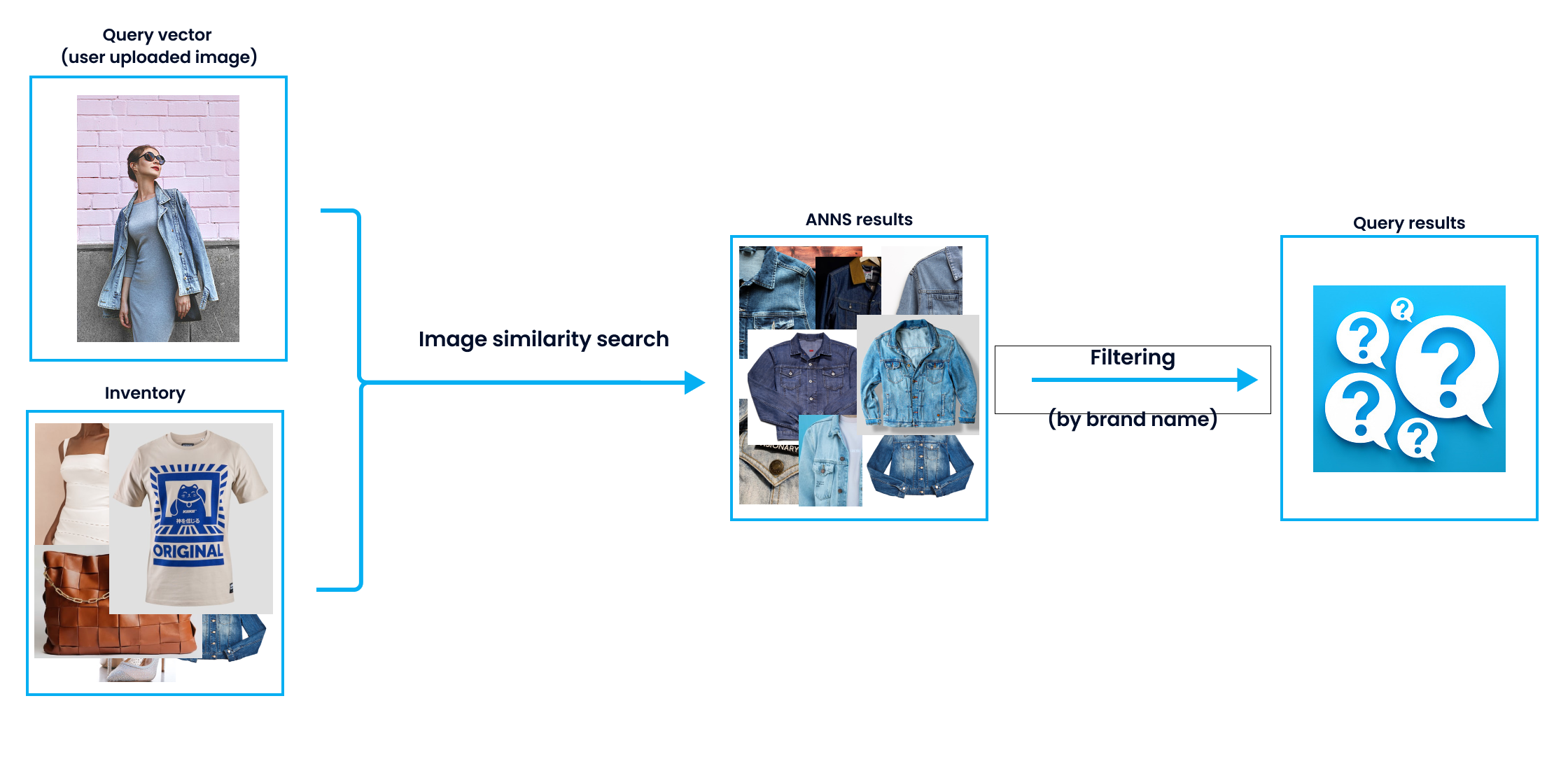
As its name suggests, post-query filtering applies filter conditions to the TopK results you obtain after a query. For instance, in the case mentioned at the beginning, the system first searches for the most similar jean jackets in its inventory. Then the results are filtered by its brand metadata.

An illustration of post-query filtering.

However, one inevitable shortcoming of such attribute filtering strategy is that the number of results whose metadata satisfying the condition is highly unpredictable. In some cases, we cannot get enough results as we wanted. Because if we want TopK (K=10) results, but after applying the filter, those vectors whose metadata does not meet the requirement will be eliminated. Therefore, we will get less hits than intended. In some worst-case scenarios, we will get no results at all after applying post-query filtering.

What if we increase the number of returned query results? We certainly can get enough results even after applying the filter condition. Nevertheless, we risk being overwhelmed by an excessive amount of results, which may burden the system as the filter condition needs to be applied to the massive similar vectors.

In-query filtering

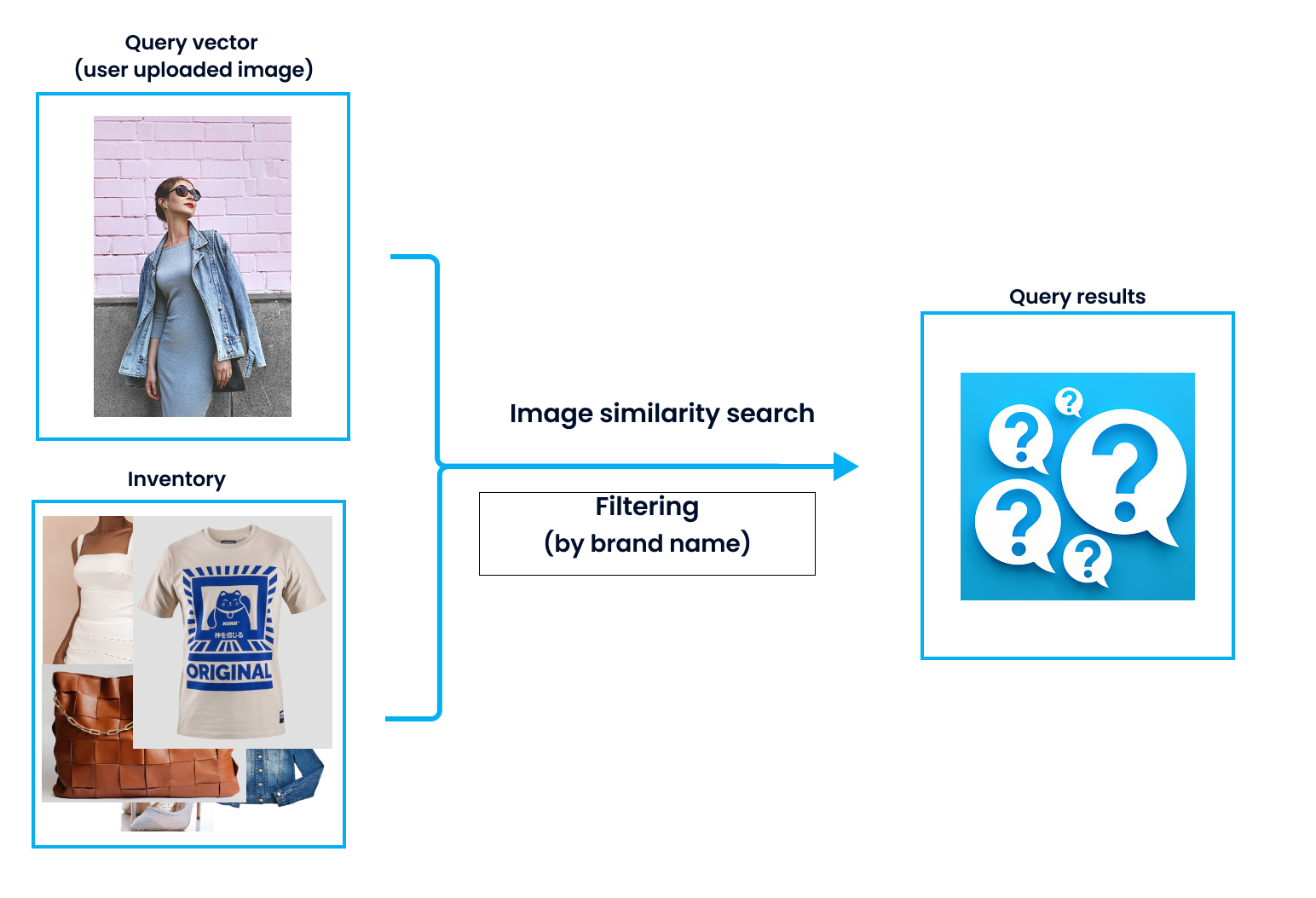
In-query filtering is a strategy in which ANNS and filtering are conducted at the same time. For instance, in the case of online shopping, images of jean jackets in inventory are converted into vectors and in the meantime, the branding information is also stored in the system as a scalar field together with the vectors. During search, both vector similarity and metadata information need to be computed.

An illustration of in-query filtering.

But an apparent shortcoming of such strategy is that it has a prohibitively high demand for the system. To conduct an in-query filtering, a vector database needs to load to memory both the vector data and the scalar data for attribute filtering. Each entity, with both vector field and scalar fields, simultaneously goes through two processes in the vector database, attribute filtering and vector similarity search. However, under some conditions, if there are too many scalar fields for attribute filtering and the usable memory is limited, you may likely encounter system OOM (out of memory).

Though one possible solution to OOM is to reduce the peak memory usage by increasing the number of segments, too many segments will lead to a worse performance of the vector database. In addition, such practice of increasing segments is not suitable for databases that store data in a column-based way as it can result in random memory access during program execution.

But on a different note, in-query filtering might be a good choice for those databases that store data in a row-based way.

Pre-query filtering

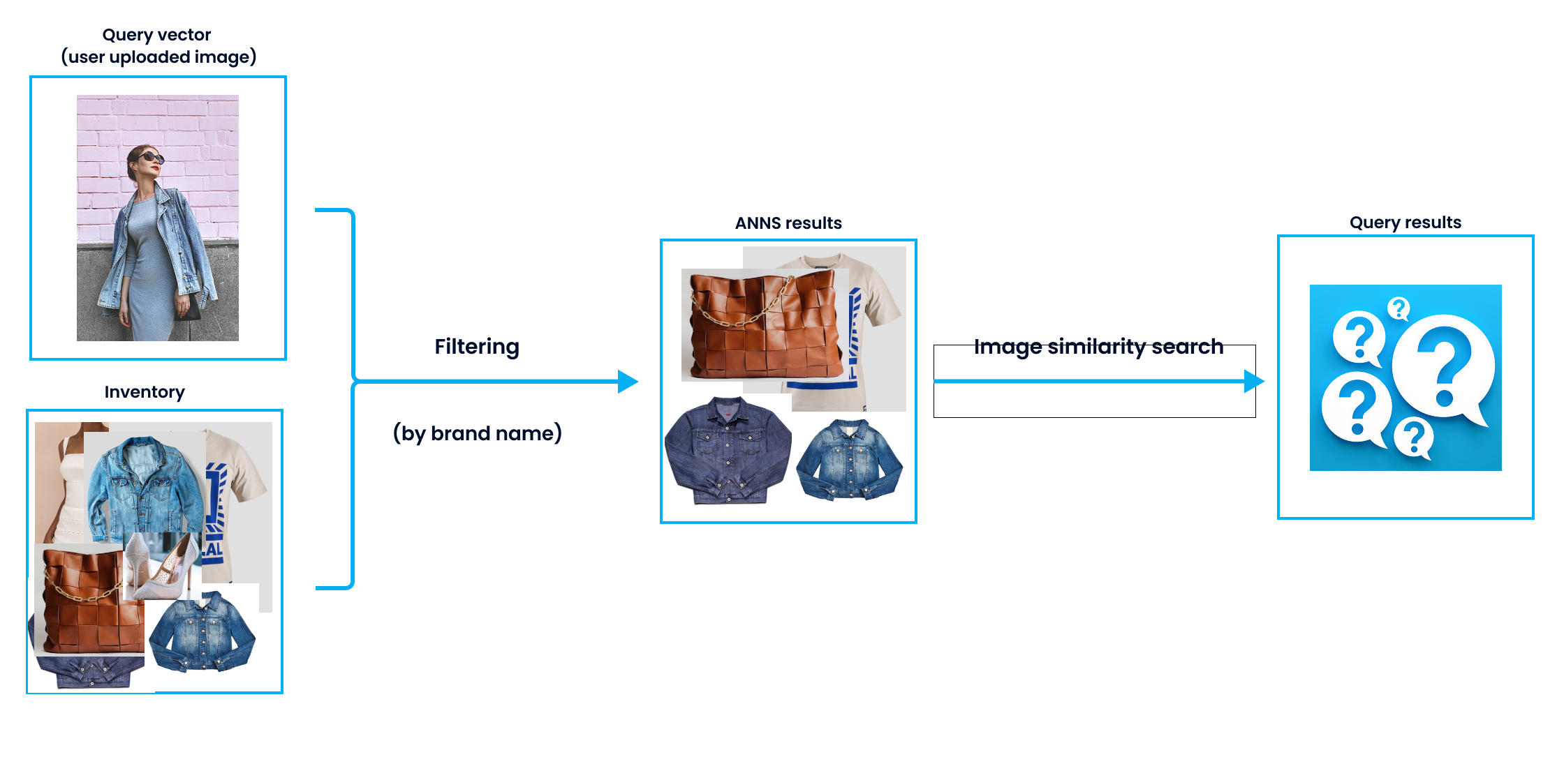
Pre-query filtering refers to applying filter conditions before ANNS. To be more specific, pre-query filtering applies filter conditions to the vector data and returns a list of results - vectors whose metadata satisfy the filter conditions. Therefore, similarity search will only be conducted within a certain scope: the eligible vectors. For instance, all jean jacket image vectors are first filtered by brand. Only those illegible image vectors will be processed during the next stage - vector similarity search.

An illustration of pre-query filtering.

Pre-query filtering sounds like a plausible solution. However, it has its own shortcoming as it slows down the search process. Since all data need to be filtered before proceeding to ANNS, the pre-query filtering strategy requires more computation. Therefore, its performance might not be as good as the other two strategies mentioned above.

An integrated attribute filtering solution

After intensive research, we discovered that Milvus, an open-source vector database provides an integrated attribute filtering solution.

The filtering strategy Milvus adopts is pretty similar to the pre-query filtering strategy but with some slight differences. Milvus introduces the concept of a bitmask to the filtering mechanism.

A bitmask is an array of bit numbers ("0" and "1") that can be used to represent certain data information. With bitmasks, you can store certain types of data compactly and efficiently as opposed to store them in Ints, floats, or chars. The bitmask works on boolean logic. According to boolean logic, the value of an output is either valid or invalid, usually denoted by "1" and "0" respectively. "1" stands for valid, and "0" for invalid. Since bitmasks are highly efficient and can save storage, they can also be used to achieve many functions such as attribute filtering, delete operations, time travel, and more.

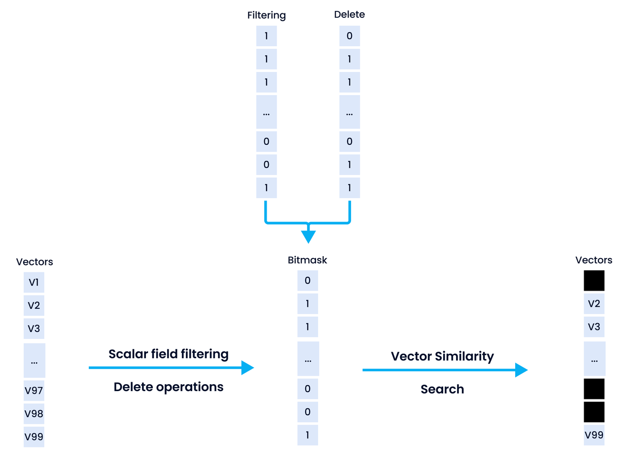
In the Milvus filtering solution, bitmask can be seen as an additional data field. If the metadata of a vector satisfies the filter condition, the vector will be marked as "1" in its bitmask field. Those vectors whose metadata does not meet the requirement will be marked as "0" in its bitmask. When all the metadata of the dataset are evaluated against the filter conditions, a bitmask only comprising of "1" and "0" will be generated. In Milvus, this filtering bitmask will be combined together with other bitmasks, such as deletion bitmask or time travel bitmask, and ultimately passed to the underlying computing engine. During ANNS, those vector data marked with "0" in the final bitmask will be ignored.

The Milvus filtering mechanism.

The Milvus filtering solution has following benefits:

• The number of results can be controlled. We are able to get the expected number of results.
• The peak memory usage is comparatively small.
• Reduce the complexity and cost of development by reusing the code for attribute filtering and other functions like delete operations as both share the same mechanism.

Filtering optimization

Despite the aforementioned solution, more work can be done to further optimize the attribute filtering mechanism.

• Two-phase computing is conducive to clearer code logic. Parallel computing can also be easily adopted to accelerate the two phases.
• Build indexes for scalar fields, especially strings, to accelerate the filtering process by greatly enhancing the efficiency of string comparison.
• Create statistics for each segment in order to quickly eliminate the entire data in the segments that do not satisfy filtering conditions.
• Build an optimizer for boolean expressions. Optimizer can transform SQL expressions to optimal execution plans that can be executed by the underlying engine. For instance, if you input the conditional expression a/4 > 100, the optimizer will turn it into a > 400, which saves the engine the trouble of dividing each value of the field a by four and compare the result with 100.
• Since in Milvus, attribute filtering is conducted before ANNS, the system performance may be hampered as each row of data needs to be filtered and computed. For IVF index, only a number of nprobe buckets are selected for computation. So if we can figure which buckets to compute, we can just filter vectors in those buckets to greatly reduce computation load. However, this optimization strategy is restricted to IVF indexes and it is not recommended to apply this kind of optimization to other types of indexes like HNSW.