Accelerating Similarity Search on Really Big Data with Vector Indexing (Part II)
Discover how indexes dramatically accelerate vector similarity search, different index types, and how to choose the right index for your AI applicatio

From computer vision to new drug discovery, many popular artificial intelligence (AI) applications are powered by vector databases. Indexing, a process of organizing data that drastically accelerates big data search, enables us to efficiently query million, billion or even trillion-scale vector datasets.
This article is a supplementary to the previous blog "Accelerating Similarity Search on Really Big Data with Vector Indexing" which covers the role indexing plays in making vector similarity search efficient, and different indexes including FLAT, IVF_FLAT, IVF_SQ8, and IVF_SQ8H. This article also provides the performance test results of the four indexes. We recommend reading this blog first.
In this article, we provide an overview of the four main types of indexes and continue to introduce four different indexes: IVF_PQ, HNSW, ANNOY, and E2LSH.
Approximate nearest neighbor search (ANNS) is an important concept in indexing. To have a better understanding of this concept and its advantage over KNN (K nearest neighbor), read the blog article written by Marie Stephen Leo.
What are the different types of common indexes?
There are numerous indexes designed for high-dimensional vector similarity search, and each one comes with tradeoffs in performance, accuracy, and storage requirements. Common index types are quantization-based, graph-based, hash-based, and tree-based. Disk-based ANNS is a product of recent advances in the area of approximate nearest neighbor search (ANNS). An introduction to this type of index will be available in a subsequent article. (Stay tuned!)
Quantization-based indexes
Quantization-based indexes work by dividing a large set of points into a desired number of clusters and ensuring that the sum of distances between points and their centroids is the smallest minimum. The centroid is calculated by taking arithmetic average of all points in the cluster.
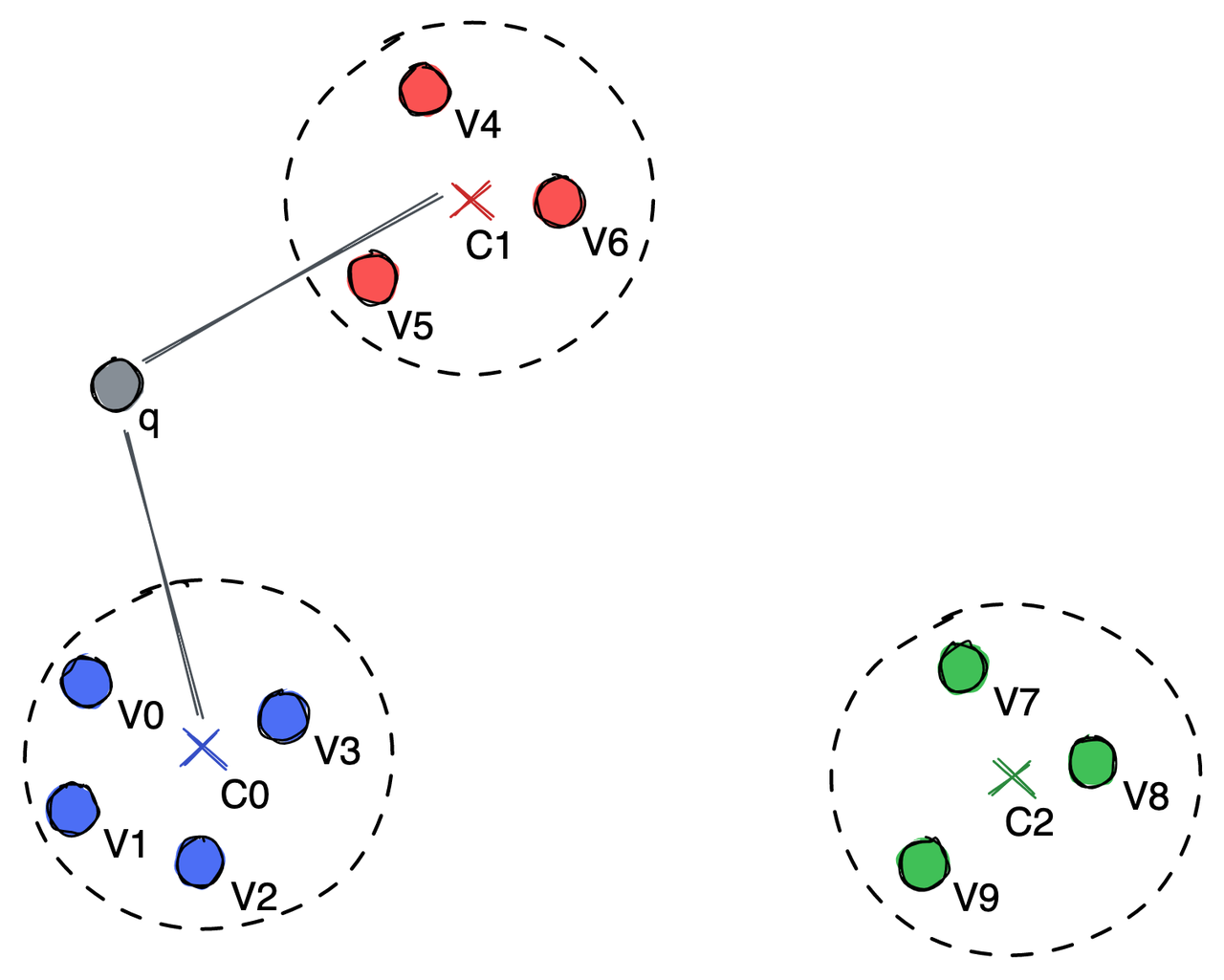
Dividing points into groups represented by a centroid.
In the illustration above, the vectors are divided into three clusters, each having a centroid point, C0, C1, and C2. To search for the nearest neighbor of the query vector q, we only need to compare the distance between q and C0, C1, and C2. After calculation, we realize that q is closer to C0 and C1. Therefore, we only need to further compare q with vectors in the C0 and C1 groups.
Graph-based indexes
Graphs, per se, contains nearest neighbor information. Take the image below as an example, the pink point is our query vector. We need to find its nearest vertex. The entry point is selected on a random basis. Sometimes the entry point could be the first vector inserted into the database. We randomly select A as the entry point for instance. B, C, D are the neighbors of A, and among them, D is the closest to the pink point. Therefore, we continue to start from D, and among its neighbors, E, F, J, the nearest to the pink point is E. However, all neighbors of E are farther compared to the pink point. Thus, we can say that E is the nearest to the pink point.
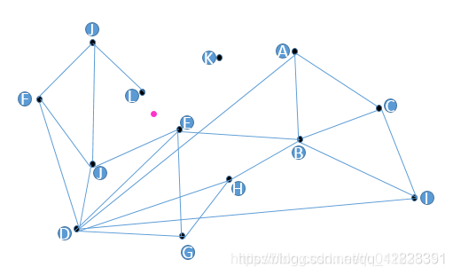
Finding the nearest neighbor of the pink point using graph-based indexes. Image source: CSDN blog.
However, there are some issues in the above approach:
- Some vertices like K are not queried.
- Vertices E and L are close to each other but not connected. So, during ANNS, L is not considered as the neighbor of E, which greatly hampers query efficiency.
- The more number of neighboring vertices to query, the larger consumption of storage. However, insufficient connection lines lead to lower query efficiency. These issues are easy to solve, as long as:
- When building a graph, all vertices need to have a neighboring vertex. In this case, vertex K can be queried.
- All neighboring vertices must be connected. (For a more detailed explanation of the connecting strategies, read Proximity Graph-based Approximate Nearest Neighbor Search.)
- The number of neighboring vertices to query can be specified via configuration.
With the issues addressed, query efficiency is still not enhanced. Therefore, we need to introduce the "expressway" mechanism here.
Expressway mechanism
Since we may start the query from an entry point that is very far away from the target query vector, we probably have to travel a really long way and go through many vertices to find its nearest neighbor. By introducing the expressway mechanism, we can skip some of the neighboring vertices to speed up the search. As shown in the illustration below, we can follow the arrows in red (the expressways) to find the nearest neighbor of the green query point. It goes through only 3 vertices.
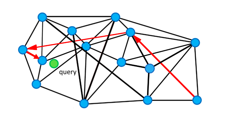
Expressway mechanism to accelerate the search.
Hash-based indexes
Hash-based indexes use a series of hash functions. The probability of a collision among multiple hash functions represents the similarity of the vectors. Each vector in the database is placed into multiple buckets. During a nearest neighbor search, to have enough number of buckets, the search radius is continuously increased. Then the distance between the query vector and vectors in the buckets are further calculated.
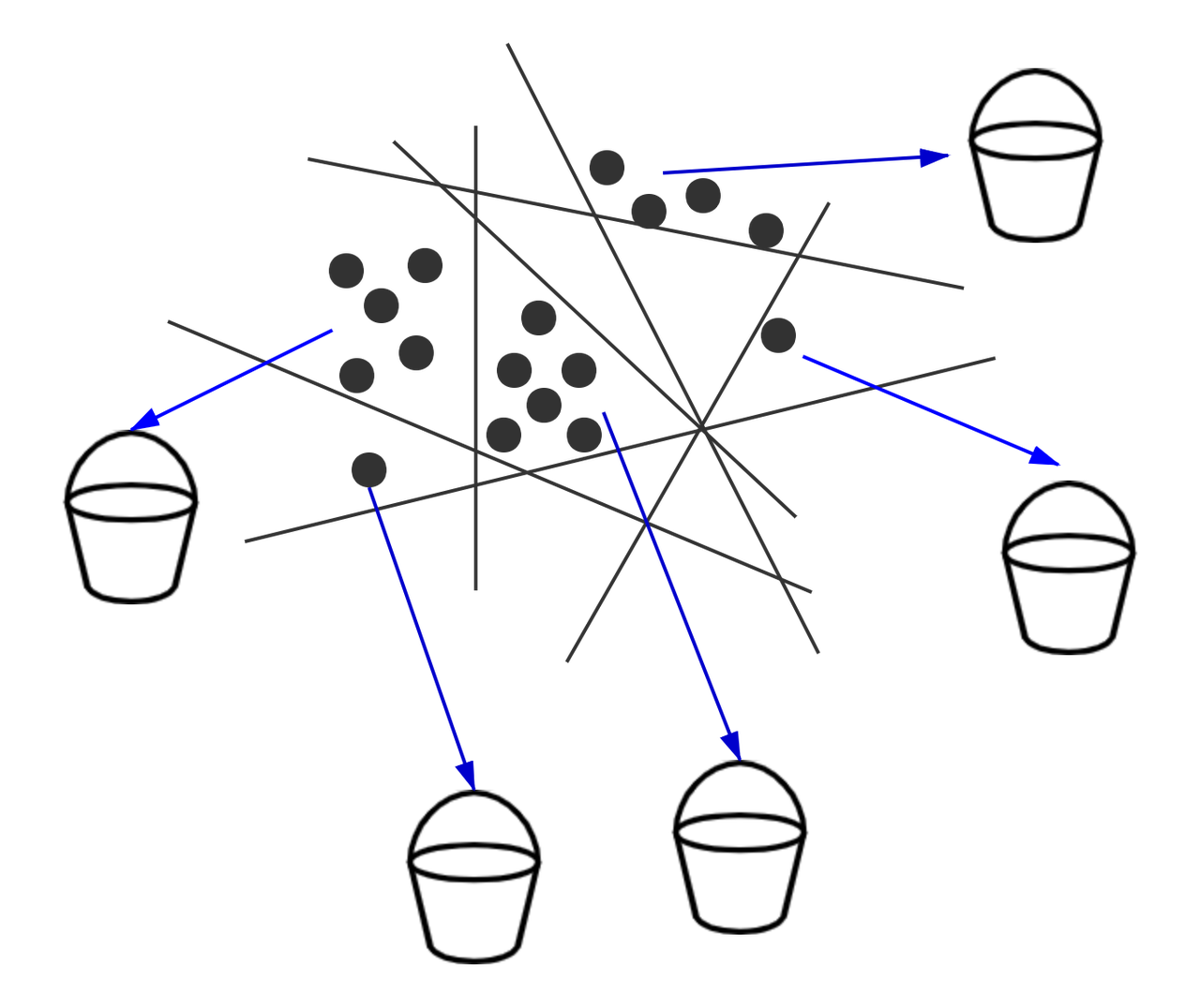
Splitting vectors into several buckets.
Tree-based indexes
Most of the tree-based indexes divide the entire high-dimensional space from top to bottom with specific rules. For example, KD-tree selects the dimension with the largest variance and divides the vectors in the space into two subspaces based on the median on that dimension. Meanwhile, ANNOY generates a hyperplane by random projection, and uses the hyperplane to divide the vector space into two.
Which scenarios are the indexes best suited for?
The table below is an overview of several indexes and their categorization.
The first four types of indexes and their performance test results are covered in the previous article "Accelerating Similarity Search on Really Big Data with Vector Indexing". This post will mainly focus on IVF_PQ, HNSW, ANNOY, and E2LSH.
| Index | Type |
| FLAT | N/A |
| IVF_FLAT | Quantization-based |
| IVF_SQ8 | Quantization-based |
| IVF_SQ8H | Quantization-based |
| IVF_PQ | Quantization-based |
| HNSW | Graph-based |
| ANNOY | Tree-based |
| E2LSH | Hash-based |
Note: Though in this post, we categorize IVF indexes as quantization-based indexes, this is still controversial in the academia as some of the researchers believe IVF indexes should not be treated as quantization-based.
IVF_PQ: The fastest type of IVF index with substantial compromise in recall rate
PQ (Product Quantization) uniformly decomposes the original high-dimensional vector space into Cartesian products of m low-dimensional vector spaces, and then quantizes the decomposed low-dimensional vector spaces. Instead of calculating the distances between the target vector and the database vectors, IVF_PQ encodes the residual vectors with a product quantizer - the difference between the vector and its corresponding coarse centroid vector. So the vectors in the database are represented by its centroid and the quantized residual vectors.
When calculating the distance between target query vector and vectors from selected buckets, IVF_PQ uses a lookup table to quickly decode the residual vector's distance.
IVF_PQ performs IVF index clustering before quantizing the product of vectors. Its index file is even smaller than IVF_SQ8, but it also causes a loss of accuracy during searching vectors.
HNSW: A high-speed, high-recall index
HNSW (Hierarchical Navigable Small World Graph) is a graph-based indexing algorithm that incrementally builds a multi-layer structure consisting of a hierarchical set of proximity graphs (layers) for nested subsets of the stored elements. The upper layers is selected randomly with an exponentially decaying probability distribution from the lower layers. The search starts from the uppermost layer, finds the node closest to the target in this layer, and then goes down to the next layer to begin another search. After multiple iterations, it can quickly approach the target.
HNSW limits the maximum degree of nodes on each layer of the graph to M to improve performance. Furthermore, a search range can be specified by using efConstruction when building index or ef when searching targets.
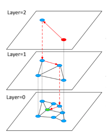
Efficient and robust ANNS using HNSW graphs.
ANNOY: A tree-based index on low-dimensional vectors
ANNOY (Approximate Nearest Neighbors Oh Yeah) is an index that uses a hyperplane to divide a high-dimensional space into multiple subspaces, and then stores them in a tree structure.
Annoy is n_tree (n_tree represents the number of trees in the forest) distinct binary trees, each node on the tree is a hyperplane subspace of the database. At every intermediate node on the tree, a random hyperplane is chosen, which divides the space into two subspaces. The leaves are the hyperplane subspaces with less than _K vectors.
As shown in the image below, ANNOY cuts the space into several subspaces. First, the space is cut into 2 subspaces.
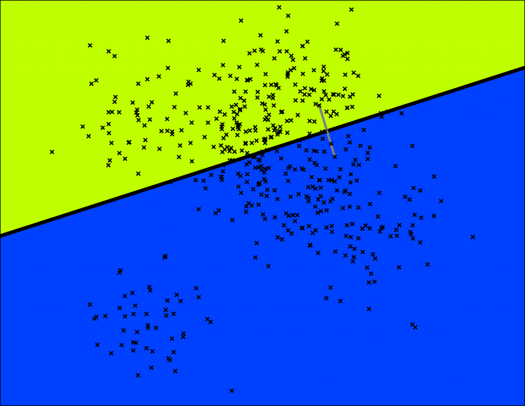
Space partitioning.
Then each of the 2 subspaces will be cut into halves, generating 4 smaller subspaces.
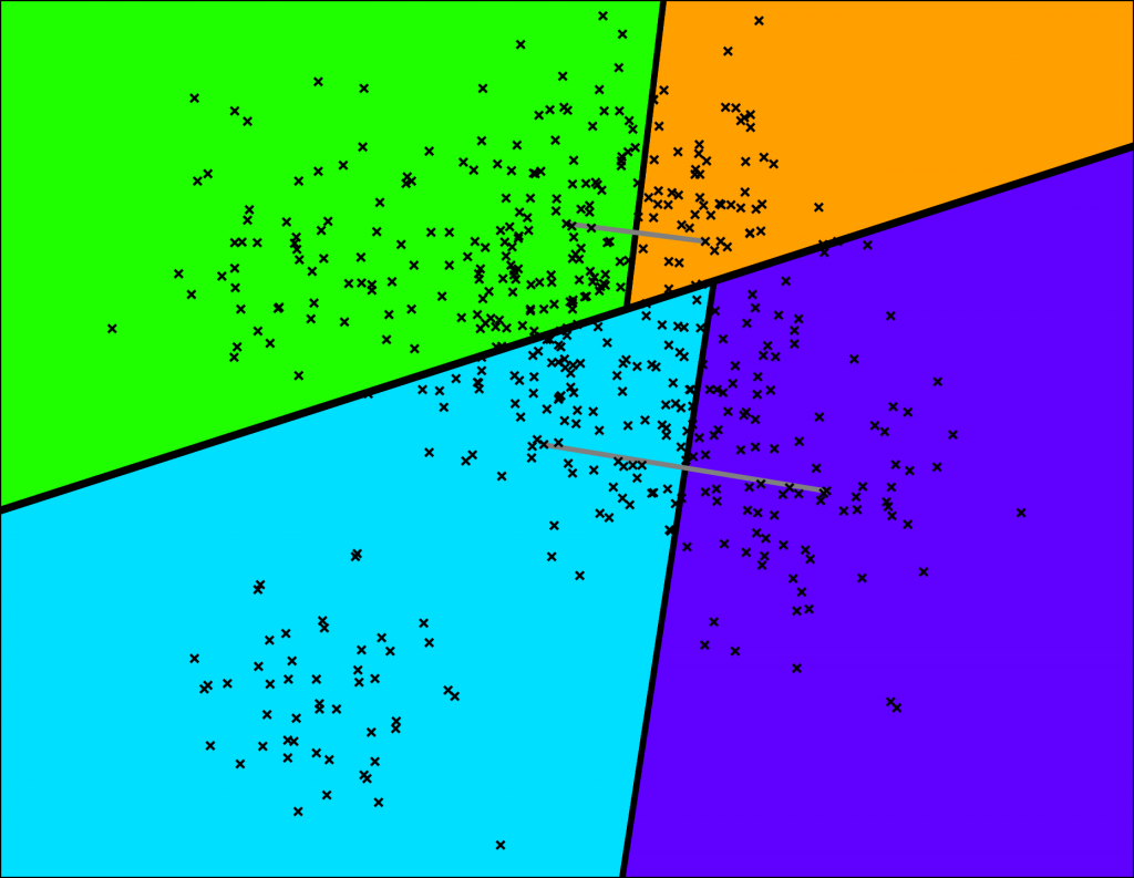
Space partitioning.
If we keep dividing the whole space, we will ultimately obtain something like the illustration below.
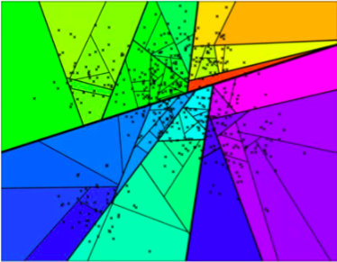
Space partitioning.
This whole process of partitioning the space resembles a binary tree.
A binary tree.
When searching for vectors, ANNOY follows the tree structure to find subspaces closer to the target vector, and then compares all the vectors in these subspaces to obtain the final result. ANNOY inspects up to search_k nodes, the value of which is n_trees * n by default if not provided. Annoy uses a priority queue to search all trees at the same time for ensuring enough nodes are traversed. Obviously, when the target vector is close to the edge of a certain subspace, it is necessary to greatly increase the number of searched subspaces to obtain a high recall rate.
ANNOY supports multiple distance metrics, including Euclidean, Manhattan, cosine, and Hamming distance. Furthermore, ANNOY index can be shared between multiple processes. However, its shortcoming is that it is only suitable for low-dimensional and small datasets. ANNOY only supports integers as data ID, meaning extra maintenance is necessary if the vector IDs are not integers. GPU processing is also not supported by ANNOY.
E2LSH: Highly efficient index for extremely large volumes of data.
E2LSH constructs LSH functions based on p-stable distributions. E2LSH uses a set of LSH functions to increase the conflict probability of similar vectors and reduce the conflict probability of dissimilar vectors.The LSH function partitions an object into a bucket by first projecting object along the random line, then giving the projection a random shift, and finally using the floor function to locate the interval of width w in which the shifted projection falls.
During search and query, E2LSH first finds the bucket where the vector object is located according to the hash function group h1, and then uses the hash function group h2 to locate the position in the bucket. The secondary hash structure of E2LSH can not only reduce the high storage overhead caused by storing the hash projection values of all vectors in the database, but also quickly locate the hash bucket where the query vector is.
E2LSH is especially suitable for scenarios where the dataset volume is large as the algorithm can greatly enhance search speed.
References
The following sources were used for this article:
- "Encyclopedia of database systems", Ling Liu and M. Tamer Özsu.
- "A Survey of Product Quantization", Yusuke Matsui, Yusuke Uchida, Herve Jegou, Shinichi Satoh.
- "Milvus: A Purpose-Built Vector Data Management System", Jianguo Wang, Xiaomeng Yi, Rentong Guo et al.
- "Efficient and robust approximate nearest neighbor search using Hierarchical Navigable Small World graphs", Yu. A. Malkov, D. A. Yashunin.
Acknowledgements
Many thanks to Xiaomeng Yi, Qianya Cheng, and Weizhi Xu, who helped review and provided valuable suggestions to this article.


